|
Interpreting null trajectories in the disorder group
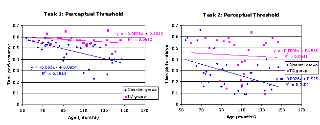
Consider the following data, drawn from one author’s studies (DA) (citation to be added). These relate to the development of perceptual thresholds in two tasks. In both cases, the TD group generates a reliable cross-sectional trajectory showing improvement on perceptual recognition. In both cases, the disorder group fails to produce a reliable trajectory, so that chronological age does not predict performance (in this case, nor did any of the mental ages derived from standardised tests deemed to be relevant to the task).
[Note that in the below figure, the groups are incorrectly captioned. Blue diamond data points are the TD group while pink square data points are the Disorder group.]

Closer inspection of the disorder trajectories for the two tasks suggests there does seem to be a difference between them. In Task 2, performance seems to be random with regard to the predictor of age: the trajectory is no more than drawing an arbitrary line through a data cloud. One might interpret this to indicate that other cognitive factors predict performance and these factors differ between the children. Let us call this pattern no systematic relationship. However, in Task 1, it seems to be more the case that the children with the disorder have prematurely reached the best level they can achieve (note the measure is still in the sensitive range; the children are not at floor performance). This looks like a real trajectory whose gradient is zero. Such a pattern would be consistent with the interpretation that the processing constraints of these children’s cognitive systems are such that development simply cannot get past a certain level of performance for the age range we are examining. Let us call this a zero trajectory, corresponding to the idea that there is zero change over time.
Unfortunately, however, despite the apparent visual difference, statistically the two cases are identical with respect to linear regression methods: the disorder group produces null trajectories in both tasks.
These two types of (theoretically different) null results appear the same statistically. Why is this? It is for two reasons. First, the linear regression model simply evaluates whether the gradient of the line is statistically different from zero. If it is not, then values of the predictor (age) are of no use in predicting values of the dependent variable (performance). They may be of no use because the dependent variable is random or because it is always the same value.
Second, and more technically, the regression equation is calculated according to the standardised residuals of the data points from the derived trajectory. In other words, although the data points for the disorder group may appear to be clustered more tightly around the flat trajectory in Task 1 than Task 2, the regression model rescales this difference so that the two flat trajectories look equally noisy.
However, statistical models depend on the assumptions built into them. In this case, because of the experimental design (a comparison between TD and disorder groups), we may add an additional assumption into the statistical model: the TD group provides us with an independent verification of the range of variability expected in the task. Therefore, we can add in the assumption that residuals need not be standardised. If we pay attention to the tighter clustering of the disorder data points in Task 1 than Task 2, it becomes possible to distinguish between the two types of null result.
The method we have developed to do this relies on rotating the data in X-Y coordinates. A flat line produces a gradient of zero. A line at 45 degrees produces a gradient of 1. If the tightly clustered trajectory is real, the R2 value should change from around zero to around 1 (for the ideal case) if the graph is simply rotated by 45 degrees anti-clockwise. However, if one rotates a random data cloud by 45 degrees anti-clockwise, it should make no difference. The cloud should still be a cloud with an flat line through it; the R2 value of the originally-null trajectory should remain close to zero. In this way, repeating the linear regressions on rotated data should distinguish between a zero trajectory and one where there is no systematic relationship.
The Excel file rotation_method_artificial_data.xls includes formulae for this transformation for two idealised cases of a zero trajectory and no-systematic-relationship. The Excel file rotation_method_real_data.xls contains an example in which these formulae are applied to a real data set in which the TD group shows a reliable trajectory but the disorder group does not; the rotation method suggests that the null trajectory is in fact a zero trajectory).
The rotation method involves 2 steps:
(1) Re-scale the trajectories so that values on both axes fall between 0 and 1. Ages are scaled to be proportions of the total age range in both TD and disorder groups; performance levels are scaled to be proportions of the total performance range in both groups. It is here where the TD group variability is used to scale the disorder group’s variability.
(2) The rescaled TD and disorder trajectories are rotated on the new axes, using the formulae
![]()
![]()
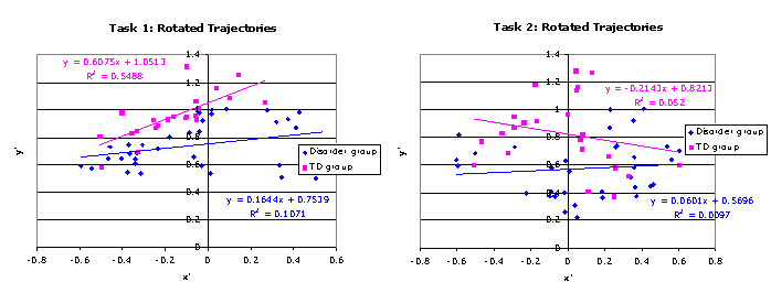
where x and y are the original x-y coordinates, x’ and y’ are the rotated coordinates, and θ is the angle of rotation in units of radians (45 degrees anti-clockwise in our case). The regressions on the rotated trajectories are shown below. For Task 1, the suspected zero trajectory, the initial R2 increases from .08 [F(1, 21)=1.86, p=.187] to a statistically reliable .55 [F(1, 21)=25.54, p<.001]. For Task 2, the suspected no systematic relationship, the R2 changes from .00 [F(1, 21)=.09, p=.772] to .05 [F(1, 21)=1.15, p=.295].
Our zero trajectory has become reliable after rotation while our no system relationship has not. Statistically, therefore, the rotation method has proved sufficient to distinguish between the two null results.
[Note that in the below figure, the groups are incorrectly captioned. Blue diamond data points are the TD group while pink square data points are the Disorder group.]

Remember, the rotation method only works because we have independent grounds for not standardising the residuals: we know the variability produced by the TD group on the same task. The rotation method would not be applicable for characterising a single trajectory; nor would it be applicable for comparing two trajectories produced by a single group, one of which is null (unless we have some strong reason to believe variability in one measure should be related to variability in a second).
Note also that the rotation method does not provide an interpretation. Where one group shows a zero trajectory and the other does not, one must ensure that this is not because one of the groups is at floor or ceiling with respect to the measure: tracing back a putative zero trajectory to cognitive developmental constraints requires confidence that the experimental task is still providing a sensitive measure of performance in both groups.
© Michael Thomas 2007
Last edited by MT 24/07/07